Abstract

This study introduces a new framework for investigating tsunami propagation and its interaction with bathymetry by decomposing total energy into kinetic and potential components. Unlike conventional approaches based on wave amplitude or energy flux, this decomposition reveals local energy imbalances that arise when a tsunami interacts with variable bathymetry. These imbalances provide a new diagnostic tool for quantifying reflection and for distinguishing regions dominated by velocity (kinetic energy) or sea-level displacement (potential energy). The method is first tested in an idealized channel with a depth discontinuity. In addition to the expected incident, reflected, and transmitted waves, an imbalance between kinetic and potential energy emerges, with its magnitude controlled by the depth contrast. This imbalance forms the basis for defining a new reflection coefficient. The approach is then applied to the 2011 Japan Tōhoku Tsunami. Results show that kinetic and potential energies remain in equilibrium during long-distance propagation but diverge near major bathymetric features such as Koko Guyot Seamount and Hess Rise, where the imbalance depends on the relative depth between the seafloor and the seamount summit. Finally, an elliptical seamount model illustrates the limitations of the method and clarifies the conditions under which energy imbalance is most relevant.

Keywords: Tsunami; Kinetic and potential energy; Energy equilibrium; Reflection at depth discontinuity; Japan tsunami 2011; Seamount tsunami interaction

1. Introduction

Tsunami waves predominantly originate from vertical seafloor motion, which imparts vertical oscillations to the ocean surface. This process initiates the conversion of potential energy into the kinetic energy of waves. The temporal evolution of kinetic and potential energy during the initial stages of tsunami generation has been detailed by Dutykh and Dias (2009) and Okal (2021). Over time, the energy conversion leads to equilibrium, where potential and kinetic energies become equal during wave propagation. Similar temporal changes occur in landslide-generated tsunamis. Analyses by Abadie et al. (2012) and Lopez-Venegas et al. (2014) indicate that energy equilibrium is disrupted within the wave-generation area and near the surface of the landslide. However, once the initial wave propagates beyond the generation zone, its potential and kinetic energies stabilize. The fundamental concepts of the temporal evolution of tsunami wave fields were formulated by Munk (1963). He emphasized that tsunami energy evolves through dispersion, refraction, scattering, and the leakage of energy from its source region into adjacent oceans. A more recent study by Fine et al. (2013) examined tsunami wave fields in the Pacific Ocean and demonstrated that the evolution of tsunami energy follows the law of energy equipartition. This was confirmed for the 2011 Japan tsunami through a combination of statistical analysis, numerical modeling, and observational data. Marchuk (2022) demonstrated the applicability of total energy derived from shallow water equations. His investigation focused on energy interactions with a conical island, assessing the proportions of wave energy reflected by the island and captured by its conical shelf. Tang et al. (2012) extensively utilized total energy concepts for the Japan Tōhoku Tsunami. They developed a method to compute the total energy transmitted by tsunami waves by combining deep ocean pressure measurements with numerical models. The source function for tsunamis was also constructed using a linear model for tsunami propagation in the deep ocean and the available computed energy. Numerous applications of this approach show that propagated energy and source location are critical for predicting tsunami impacts. Understanding how tsunami energy evolves over time, particularly its decay rate, is crucial for tsunami prediction and warning. Based on tsunami gauge recordings during a recent megatsunami in the Pacific, Rabinovich et al. (2013) estimated the mean energy decay time to range from 17 to 25 hours. The rate of decay depends on the tsunami wave frequency; shorter period tsunamis decay faster, while longer period tsunamis decay more slowly. The mechanism of transmitting tsunami energy from its source to various global ocean regions can be investigated through energy flux, a key term in the energy balance equation, see Kowalik (2008). Energy flux contours applied to the Kurile Islands Tsunami of 2006 (Kowalik et al., 2008) and the Japan Tōhoku Tsunami of 2011 (Horrillo et al., 2012; Tang et al., 2012) identified Koko Guyot and Hess Rise as critical bathymetric features responsible for scattering and refocusing tsunami signals. The time history of energy fluxes demonstrated that waves scattered from Koko Guyot were the cause of the late arriving maximum observed wave amplitude at Crescent City approximately two hours after the arrival of the initial wave. By integrating the energy flux over time, Yoon et al. (2014) introduced the concept of net energy flow per unit width during a given time interval. This approach made it possible to clearly establish the connection between tsunami sources and sinks. The net energy flow revealed how submerged rises and ridges capture tsunami energy and channel it toward coastal areas. The application of the energy conservation and the variability of potential and kinetic energies to study tsunami runup and rundown was successfully demonstrated by Li (2000) and Zhao et al. (2012). The interaction of tsunamis with prominent bathymetric features is often linked to wave reflection, transmission, and scattering, see Mofjeld et al. (2000). Their analytical theory, based on linear long-wave equations, examined tsunami wave scattering by idealized topography. This research also introduced a scattering index to estimate regions where ocean bathymetry significantly scatters tsunami waves (Mofjeld at al., 2001). The index is based on the relative depth between the ocean floor and the top of the bathymetric feature. Given that numerical models provide the distribution of kinetic and potential energy at each time step, the objective of this study is to evaluate the use of local kinetic and potential energy imbalance to investigate the evolution of tsunamis over spatially varying bathymetry. The following Sections 2 and 3 introduce the equations of motion and the corresponding energy-conservation relations, with particular emphasis on energy fluxes in progressive and reflected waves. Section 4 presents numerical experiments of wave propagation in a channel with a bottom break, demonstrating how the energy-based reflection coefficient relates to the resulting interference pattern. Section 5 describes the 2011 Japan Tōhoku tsunami. Temporal relationships between kinetic and potential energies are examined in Section 6 and in Subsections 7.1 and 7.2. To reproduce and emphasize the key findings, Subsection 7.3 employs a simplified model of an elliptical seamount. Section 8 summarizes the results and discusses broader applications of energy-based diagnostics.

2. Equations of motion and continuity

While the equations of motion, continuity, and energy conservation are well known, it is helpful to repeat them here to define notations and units, especially for kinetic and potential energy and various forms of energy flux. Equations used in tsunami study are the long waves (shallow water). Only horizontal (vertically averaged) velocity components $u$ and $v$ are considered in these equations. Shallow water equations of motions along the $x$ (pointing eastward) and $y$ (pointing northward) coordinates take the following form, see Horrillo et al. (2021),

and

The equation of continuity for the vertically averaged motion is defined as,

In the above equations: $u$ and $v$ are the velocity components, $\zeta$ is the sea level, $D$ the depth, $\rho$ the density, $f$ the Coriolis parameter, $\tau^s$ the surface stress, $\tau^b$ the bottom stress, and $N_h$ the horizontal eddy viscosity. Bottom stress is a function of current and is frequently formulated as

with dimensionless drag coefficient $R$ in the deep water set to about 0.003.

3. Energy equation

The energy equation, is related to the physics of tsunami generation, propagation, and dissipation. This equation can be derived from the above equations of motion and continuity, see Horrillo et al. (2021),

In this form, Eq. (5) can be seen to be a specific case of the general statement of conservation of energy. The first term on the LHS is the time rate of change of kinetic energy plus potential energy density, defined here as the rate of change of energy stored within a fluid column of unit surface area, centered on the point $x$,$y$, and extending from the ocean bottom $-H$ to the surface $\zeta$. The units are, therefore, power per unit area. The potential energy density, $e_p=\rho g\zeta^2/2$, arises from the work required to build a mound of sea water of unit area and $\zeta$ meters above mean sea level. The kinetic energy density is defined by the product of fluid column depth times current magnitude squared, so $e_k=D\rho(u^2+v^2)/2$. The terms on the RHS of Eq. (5) are source terms. From left to right, these are power inputs from bottom and surface stresses and horizontal friction. Bottom and surface stresses are due to bottom friction and wind stress. Wind stress is usually neglected in the study of tsunamis, as tsunami energy dissipation occurs mainly through the action of bottom friction. The remaining two terms on the LHS of Eq. (5) are identified as energy transport into and out of the fluid column. They can also be viewed as the divergence of an energy flux vector, $\mathbf{E}_h$, which is expressed in the Cartesian coordinate system as

The first order approximation (not valid in very shallow water), is

It is often used to describe the transfer of energy from point to point. Note that just as in the derivation of Eq. (5), the Coriolis terms have been dropped out. The above formulas can be simplified by considering frictionless propagation of the linear wave propagating in the positive x direction, see Kowalik and Murty (1993). In progressive long waves the sea level

and the velocity are connected by the following expression,

Introducing the above expressions into eq. (6a) for the energy flux, the energy flux reads, see Nekrasov (1992)

The energy flux of the progressive wave is always positive and it changes from zero to $\rho g\sqrt{gH}\zeta^2_a$. It is aligned with the direction of propagation, but not with velocity which can be positive and negative, it propagates in the same direction as the sea level and velocity, and its period of propagation is twice as short as that of the sea level or velocity. The maximum sea level does not require the knowledge of velocity. For the full calculation using Eq.(9) one can apply observational sea level data from buoys or coastal gauges, see Koshimura et al. (2008). The general solution in the channel is a superposition of two waves running in positive and negative $x$ directions. Considering incident and reflected wave in the channel,

The above amplitudes can be connected by the reflection coefficient $r=\zeta_b/\zeta_a$,

and the associated velocity is

Energy flux in this combined wave, computed according to the first term in Eq. (6a)

is a sum of progressive wave (see eq. 9) and standing wave fluxes, the result of the superposition of two waves. Treating the energy flux as a vector, the analogous expression for the second horizontal component is obtained by replacing $x$ with $y$ and $u$ with $v$. The value of the energy flux in both the progressive wave and the standing wave depends on the reflection coefficient, r. As a standing wave has half the wavelength of the progressive wave, the energy flux in the standing wave is changing at the quarter wave length between nodes where velocity and kinetic energy are at maximum, and antinodes where sea level and potential energy are at maximum. In the standing wave there is no net energy propagation over time. Only the energy is fluxing over one quater wavelenth from kinetic to potential energy and vice versa. Therefore the energy is switching between kinetic and potential over a quarter wavelength. The two energies oscillate out of phase with one another. The variable energy fluxes ought to be related to the difference in the kinetic and potential energy when the progressive and standing wave occur together. For simplicity the amplitude and velocity are rewritten as sum and difference of two terms, see Lamb (1945).

Here $A$ denotes incident and $B$ reflected wave. With the help of the above solution, the potential and kinetic energy are defined as,

The interaction between the two waves is expressed by the interference term $(AB)$. Without this term, the potential and kinetic energies remain equal at every time step. The interference term introduces variability into the kinetic and potential energies. It varies over time due to the interaction between the incident and reflected waves, leading to fluctuations in the kinetic and potential energy values. When the trough of the incident wave aligns in phase with the trough of the reflected wave, potential energy dominates. Conversely, when kinetic energy dominates, the combined sea level of the incident and reflected waves is minimal. If the incident and reflected waves become separated, the interference process ceases, and the kinetic and potential energies return to their equilibrium states. The interference term also highlights significant deviations from the equality of potential and kinetic energies during the process of wave reflection at a topographic discontinuity. The magnitude of these deviations correlates with the strength of the interference term, which depends on the amplitude of the reflected wave $B$. This amplitude, in turn, is influenced by the depth difference between the oceanic floor ($H_d$) and the top of the bathymetric feature ($H_s$). As described in Eq. (13), the interference term evolves over time, reflecting the energy transfer between maximum kinetic energy and maximum potential energy, and vice versa. According to Eq. (15), the maximum difference between potential and kinetic energy is given by $g2\,\mathrm{Max}(AB)$. The relative strength ($r_i$) of this term defines the reflective properties of the topographic discontinuity.

The coefficient $r_i$ varies within the range $0\leq r_i\leq 1$. Along a smooth bottom, where $e_p=e_k$, $r_i=0$. At a vertical wall, where $u=0$, $e_k=0$, $r_i=1$. The purpose of this research is to apply the above energy relation to study the interaction of tsunamis with bathymetry.

4. Numerical experiments in the channel of 4500 m and 500 m depth with an interconnecting depth break

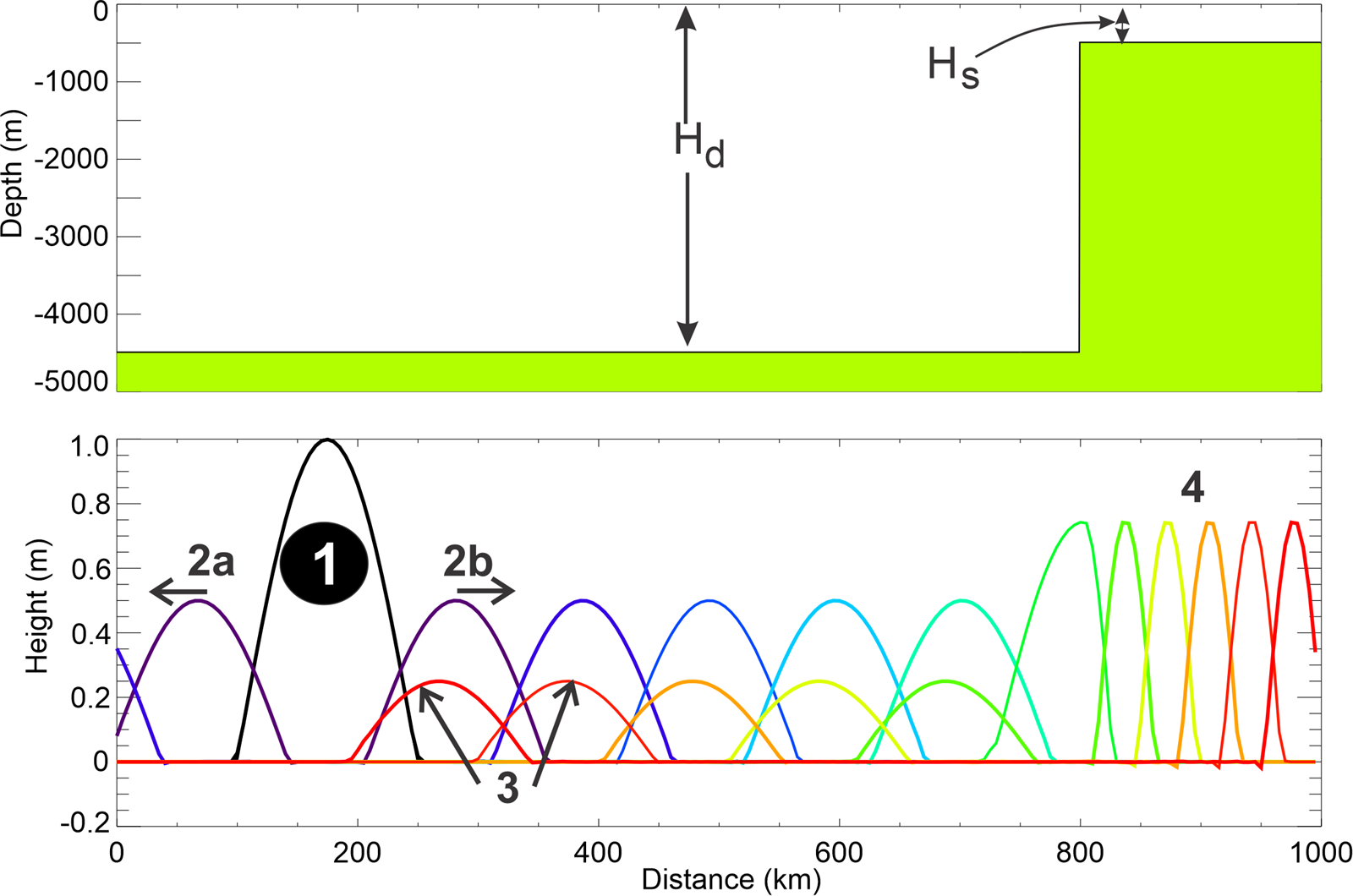
This numerical experiment simulates wave propagation in a 1000 km-long channel. At 800 km from the left boundary, the channel's depth changes abruptly from 4500 m to 500 m. Right of this depth transition, the new constant depth continues for 200 km, as shown in the upper panel of Figure 1. For future reference, the depth in the deeper portion of the channel is denoted as $H_d$ and in the shallow portion $H_s$. The simulation does not include bottom friction ($R=0.0$) or nonlinear terms. A short spatial step of 500 m and a time step of 0.1 s are chosen in the numerical solution to resolve all the details of the wave propagation.

The equations of motion and continuity used in this experiment are as follows,

The energy equation is,

The initial instantaneous displacement of the free surface is defined as a half-sinusoid with a height of 1 m. This displacement, spanning a length of 150 km, is located between 100 km and 250 km, and its period is 11.9 min. Figure 1, lower panel, illustrates the time history of wave propagation within the channel. The initial displacement subdivides into a pair of waves, each 0.5 m height, propagating to the left (2a) and the right (2b). The leftward moving wave exits the channel, while the rightward moving wave is shown at various times with different colors as it propagates along the channel. The wave's shape remains well-preserved within the deep section of the channel (first 800 km). Impinging on the abrupt bottom change, where the bottom rises from 4500 m to 500 m, the wave is partially reflected to the left (3), while the transmitted right-going wave continues into the shallower section (4). The wave in this shallow domain is symmetrical; however, due to the reduced depth, its height increases and its wavelength shortens relative to the deeper region.

To study the evolution of energy over time, one can observe how a wave passes through a fixed point in the numerical grid. Kim and Son (2018) proposed a more effective approach: integrating potential and kinetic energy along the channel at each time step. This method tracks the wave's leading front, providing a clearer picture of energy evolution. In Figure 2 (upper panel), this approach is applied to show the time history of potential and kinetic energy. At the initial moment (1), all energy is stored as potential energy, represented by the brown line with diamonds. The channel integration at this stage yields 73.6 joules. As the wave begins to propagate, potential energy decreases, while kinetic energy, as shown by the blue line, increases—reflecting the conversion of potential energy into kinetic energy as particles begin to oscillate. Approximately six minutes after the start, when the two waves (2a and 2b in Figure 1) are fully separated, equilibrium is reached (stage 2), with both potential and kinetic energy equal to 36.8 joules. From stage 2 to stage 3, the total energy diminishes as the left-going wave (2a) exits the channel through the open left boundary. During the interval marked as domain 3, potential and kinetic energy remain balanced at 18.4 joules, indicating steady rightward propagation of the remaining wave. However, when the wave encounters an abrupt change in depth, leading to partial reflection, the interaction between the incident and reflected waves creates an interference pattern in the energy plot (4). The largest disparity between potential and kinetic energies occurs when the crest of the incident wave aligns with the crest of the reflected wave, causing a peak in potential energy and a corresponding minimum in kinetic energy. In time domain 5, equilibrium is reestablished. During this period, the propagation involves the rightward-moving wave in the shallow part (4 in Figure 1) of the channel and the leftward-moving reflected wave in the deep section (3 in Figure 1). In domain 6, only the reflected wave in the deep channel remains, while the forward-propagating wave in the shallow region has exited the channel. The energy flux shown in Figure 2 (lower panel) reflects the stages outlined in the energy plot above. Although a positive energy flux indicates rightward propagation, it does not necessarily imply that all waves are traveling rightward. Initially, during the energy transformation phase (1–2), the energy flux remains close to zero. The increase in energy flux corresponds to the propagation of two waves (Figure 1, 2a and 2b), eventually resulting in a single rightward-traveling wave (3) that produces a constant, elevated energy flux. In the time domain 5, the lower energy flux results from the interaction of the reflected wave in the deep channel (negative flux) with the rightward-moving wave in the shallow channel. In the time domain 6, as the wave in the shallow domain has exited, the energy flux turns negative, indicating that only the reflected wave in the deep region continues to propagate.

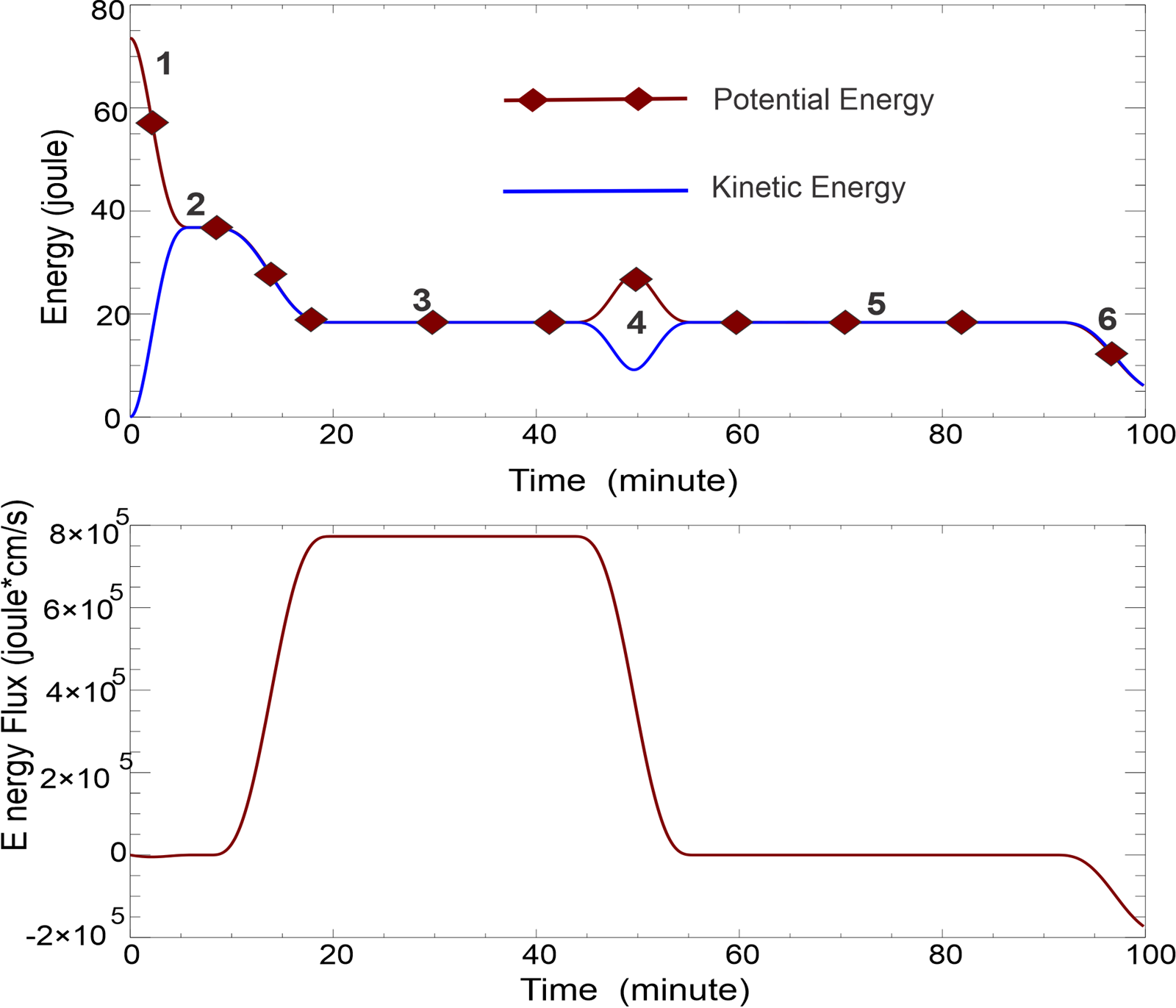
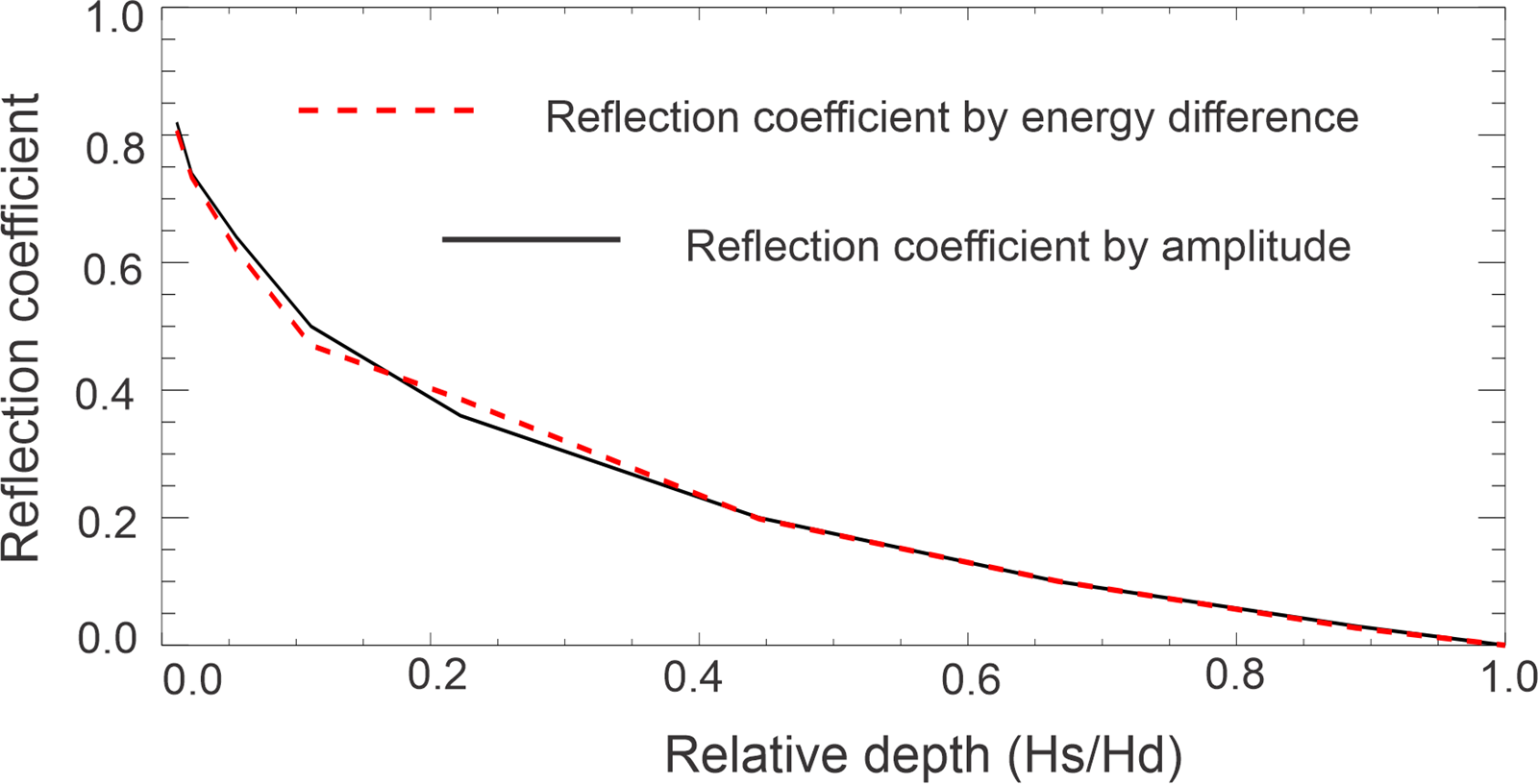
A significant result of this numerical experiment is the observed relationship between potential and kinetic energy. During wave propagation in both the deep and shallow sections of the channel, potential and kinetic energies remain equal, indicating an equilibrium state. This equilibrium, however, is disrupted when the wave encounters the abrupt change in bottom depth. Notably, equilibrium is quickly re-established afterward as the wave continues to propagate along the channel. An estimate of the time required to reach this equilibrium can be made based on the initial phase of wave generation. Figure 2 shows that approximately 6 minutes are needed to achieve equilibrium following the initial sea level disturbance. This time corresponds to a distance of approximately 75 km, which the signal travels at the phase velocity. Thus, the time required for energy equilibrium to be reached in the channel suggests that this state is attained when the signal has traveled only half the initial length of the free surface disturbance. This is also the time the two waves (2a and 2b, as shown in Figure 1) are fully separated. In the next set of numerical experiments, wave reflections is investigated at the vertical bottom break by varying the depth in the shallow part of the channel ($H_s$) relative to the deep portion ($H_d$). This variation allows to derive the classical reflection coefficient, as detailed in Mei et al. (2005) and in Levin and Nosov (2015). Additionally, a new coefficient, $r_i$, is introduced defined by the maximum of the absolute difference between kinetic and potential energy at the bottom break, see Eq. (16). This coefficient, along with the classical reflection coefficient, will be plotted as a function of relative depth.

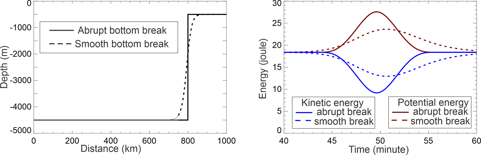
In Figure 3, the shallow depth $H_s$ varies from 500 m to the deep depth $H_d=4500$ m, with relative depth defined as $H_s/H_d$. The coefficient $r_i$ is calculated according to Eq.(16). To illustrate this, refer to Figure 2, where $H_s=500$ m, $e_p-e_k=17.3$ joule, and total energy 2*18.4 joule, therefore $r_i$=0.47, while the reflection coefficient (r) calculated as the ratio of reflected to incident wave amplitudes, equals 0.5. Figure 3 shows that the traditional reflection coefficient based on wave height (or amplitude) is well correlated with the coefficient based on the energy difference. This correlation indicates that the reflection coefficients are connected to the energy imbalance at the bottom features. Our goal is to explore this imbalance in energy distribution as a potential indicator for identifying regions of tsunami-ocean bottom interaction. In tsunami propagation studies, it is relatively straightforward to measure the incoming wave amplitude, but defining the reflected wave amplitude is more challenging. By tracking both kinetic and potential energy in the computational process, a new metric is added to evaluate the reflective properties of bottom features. Before advancing to ocean-wide tsunami propagation, different interference patterns are examined through different bottom profiles. Figure 4 (left panel) shows two bottom profiles: one an abrupt change from 4500 m to 500 m, and the other a smooth gradient indicated by the dashed line. In the right panel, the energy interference patterns in the time domain are illustrated as the wave interacts with these bottom changes. For the smoothed bottom transition, the maximum difference between potential (brown, dashed line) and kinetic energy (blue, dashed line) reduces to 10.8 joules, compared to 17.3 joules for the abrupt change. The reflection coefficient is $r_i=0.29$, and the amplitude reflection decreases to $r=0.26$. The amplitude of the reflected wave (not shown here) reduces to 0.13 m, while the disturbance extends over 300 km from its original 150 km in the incident wave. The differences in interference patterns for the smooth bottom profile arise from an extended reflection process over time. The initial signal encounters deep water, where the phase velocity is high. However, as it progresses up the slope, the phase velocity decreases, slowing and lengthening the interaction. Consequently, the reflected wave develops a steeper, shorter frontal lobe and a longer, slower-moving tail. This behavior is evident in the interference pattern, where a shorter initial signal is followed by a prolonged signal arriving after the peak in potential energy, as shown in Figure 4. Similar behavior has been observed in energy transformations in the time series of potential and kinetic energy in the runup and rundown processes of a solitary wave, as noted by Li (2000) and Zhao et al. (2012). When the wave reaches the shore, it exhibits energy equilibrium. During the runup, the energy level is amplified, with potential energy dominating over kinetic energy. Conversely, at the rundown, the reverse process occurs: kinetic energy increases while potential energy decreases until equilibrium is restored.

The above specified bottom bathymetry with the sharp break is applied to study the behavior of a sinusoidal wave, which commonly represents tsunami waveforms generated by earthquake-induced seafloor deformation, where uplift and subsidence combine to create the initial wave. A sinusoidal free-surface deformation with a wavelength of 150 km is positioned in the deep section of the channel and propagates toward a bottom break.

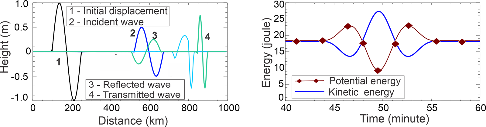
In Figure 5, the initial free surface disturbance (1), with an amplitude of 1 m, generates an incident wave (2, blue) of 0.5 m in the left panel. Upon reaching the bottom break, the wave partially reflects (3, green) and travels back toward the left end of the channel and is partially transmmited into the shallow domain (4, green). Notably, the incident wave moves to the right with a leading edge depression, and after reflection, it propagates leftward still with a leading negative sea level. As a result, when the incident and reflected waves interact at the bottom break, the negative sea level is initially amplified, producing a potential energy peak at around 46 minutes (right panel). The minimum sea level corresponds with a kinetic energy peak, and when positive sea levels interact, a new potential energy maximum occurs around 53 minutes. The maximum difference between kinetic and potential energies at 49.5 minutes is 19.5 joules, yielding a reflection coefficient of $r_i=0.53$, while the amplitude reflection coefficient is $r=0.5$.

5. Japan Tōhoku Tsunami of 11 March 2011

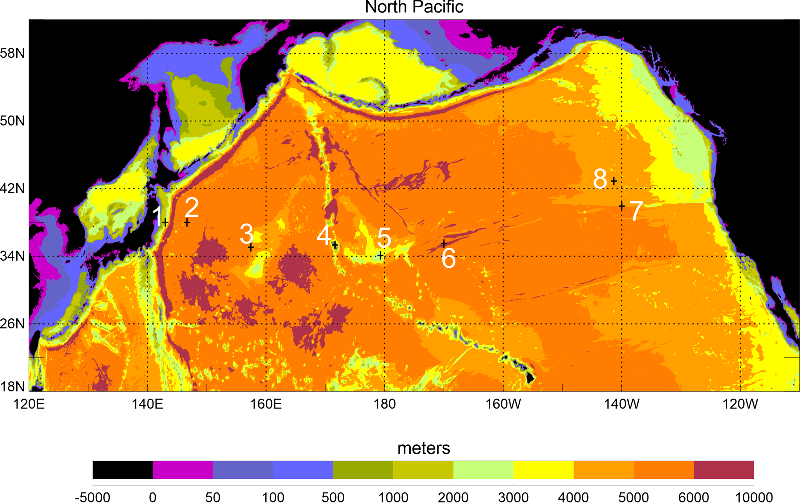
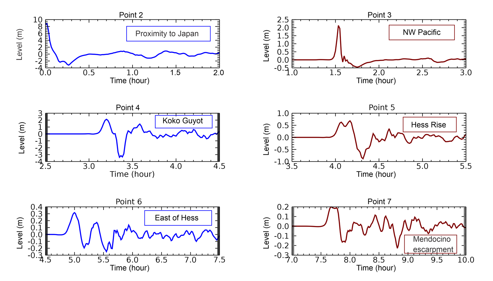
This investigation focuses on energy distribution in the Japan Tōhoku Tsunami of March 11, 2011. The tsunami signal will be analyzed at several points between the source and Koko Guyot (KG), and along its route to Crescent City via the Mendocino Escarpment. Figure 6 illustrates the bathymetry of the North Pacific used in our computations, based on data from the British Oceanographic Data Centre (2003). The numbers indicate points of signal recording and analysis. The source of the Japan tsunami is modeled using the formulations of Okada (1985) with parameters described by Horrillo et al. (2012, 2021). The tsunami simulations are carried out with the Global Tsunami Model, which was previously applied to the 2004 Indian Ocean Tsunami (Kowalik et al., 2005) and the 2006 Kurile Islands Tsunami (Kowalik et al., 2008). The step-by-step construction of the model, as well as the relationship between numerical errors (numerical dispersion and friction) and tsunami physics, are discussed in detail by Horrillo et al. (2021) and Kowalik and Murty (1993). The model computations, performed in a spherical coordinate system, simulate 30 hours of tsunami propagation, allowing the signal to traverse the entire North Pacific. Figure 7 presents the sea level signals of the tsunami as it travels between Point 2 (near Japan) and Point 7 (Mendocino Escarpment). A narrow positive peak, followed by a smaller amplitude negative wave, travels from the source region (Point 2) through the North Pacific (Point 3) to KG, without significant changes in wave characteristics. Upon reaching KG seamount (Point 4), the sea level signal changes in periodicity and character, with the negative peak reaching a pronounced amplitude of nearly 3 meters. KG transmits the tsunami signal to Hess Rise (Point 5), where both the periodicity and amplitude of the sea level signal are further altered. At Point 6, located east of Hess Rise (HR), the signal displays positive and negative oscillations, which undergo additional transformations as it travels toward the Mendocino Escarpment (Point 7).

The maximum tsunami amplitude at each grid point was recorded during this computation. The amplitude represents the positive sea-level change from the mean sea level to the wave crest. Figure 8 illustrates the maximum amplitude within the North Pacific domain. The tsunami signal generated by the source near Tōhoku propagates as a positive wave toward the southeast Pacific and as a negative wave toward the Japan Sea. Some tsunami energy propagates in a finger-like pattern, which is a result of wave refraction and refocusing around chains of islands, seamounts, and passages. A closer analysis reveals that the strong directionality of the tsunami, influenced by the elongated source, dominates its propagation. However, this directionality is locally disrupted by maxima caused by interactions with bathymetric features. The details of these interactions are clearly depicted in Figure 8.

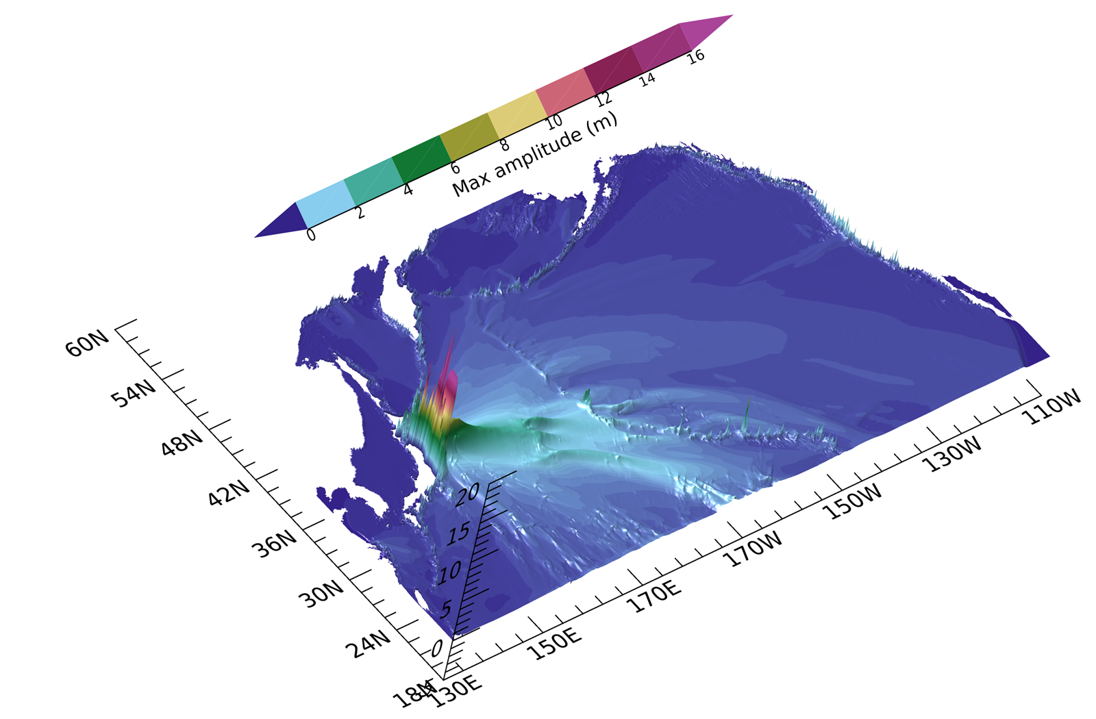
The maxima along the primary energy lobe result from interactions with the Emperor Seamount Chain, and particularly with two prominent bathymetric features: KG and HR, located at the southern tip of the chain. Smaller spikes of energy are attributed to interactions with the Hawaiian Ridge. The finger-like pattern of the energy lobe, as shown in Figure 8, can be clearly associated with significant bathymetric features, see Tang et al. (2012) and Horrillo et al. (2012). For example, the maximum energy directed toward Crescent City is linked to the Mendocino Fracture Zone. The maximum amplitude distribution indicates two distinct types of tsunami wave propagation: a relatively smooth signal change across vast oceanic areas and abrupt changes when a tsunami encounters prominent bathymetric features. To better understand the interaction between an incoming incident wave and significant bathymetric features, the presence or absence of energy equilibrium is analyzed. The lack of equilibrium corresponds to a strong interaction between the wave and the obstacle.

6. Temporal relation between kinetic and potential energies

First, in this section, the energy is analyzed to observe the transoceanic propagation of the tsunami wave.

Figure 9 illustrates the temporal relationship between potential and kinetic energy at four distinct points. The analysis begins at the tsunami source located at 143°W, 38°N (Point 1 in Figure 6), proceeds to a nearby location at 146.67°W, 38°N (Point 2, 322 km from the source), continues to a point in the northwest Pacific at 157.4°E, 35°N (Point 3), and concludes at Koko Guyot (Point 4).

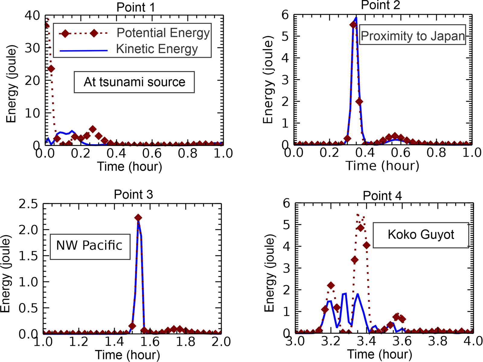
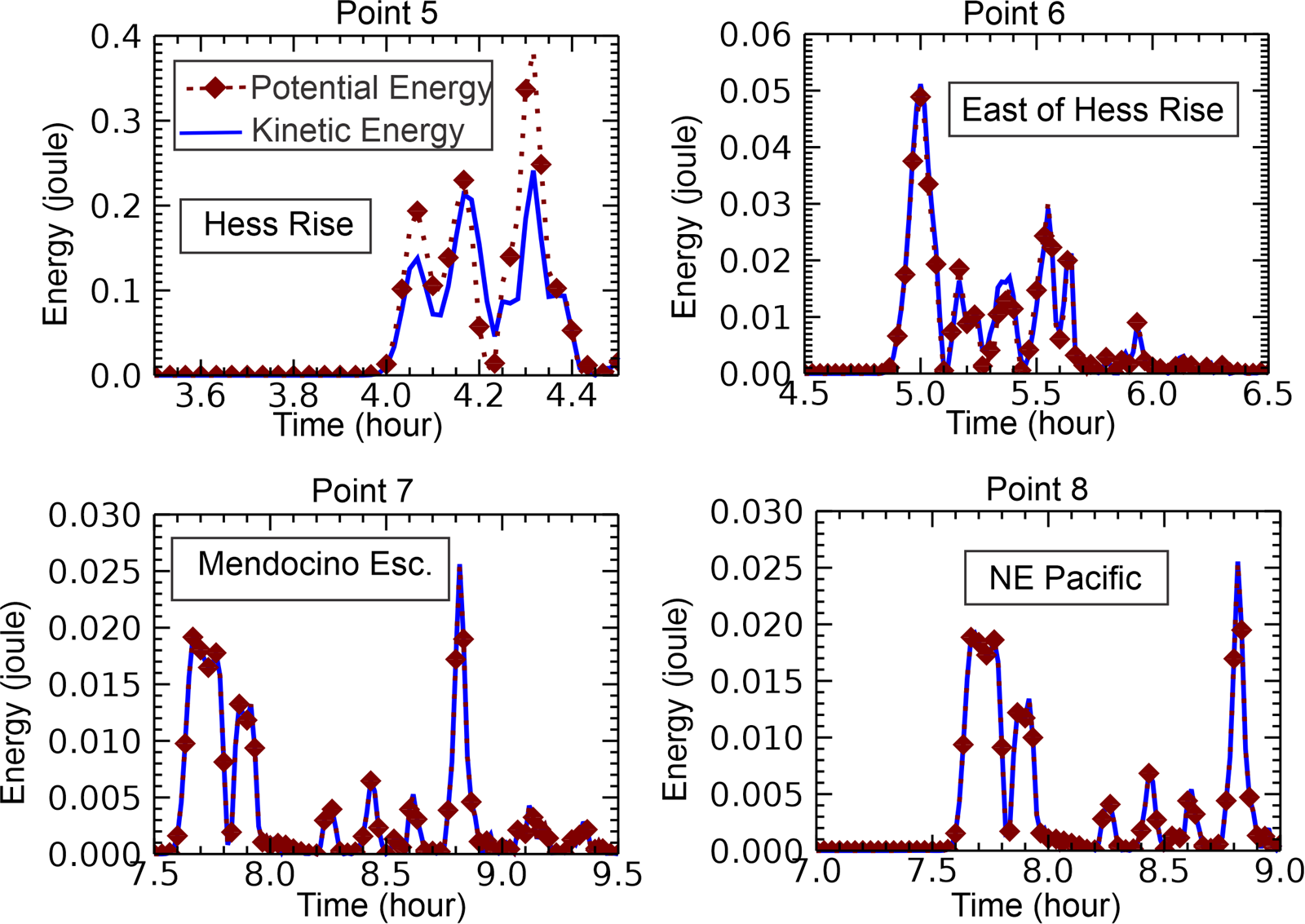
The behavior of the energy at the source shows the dominance of the potential energy, while the kinetic energy is just starting to grow. At the point located 322 km from the source, the energy equilibrium is already established, and this mode of energy transmission continues up to KG. Here, equilibrium is broken, and the energy changes in time in a new way, different from the open ocean. Hence, this energy plot confirms the strong interactions between the tsunami and the KG bathymetry. Figure 10 depicts energy, starting from the HR (Point 5, in Figure 6, at a depth of approximately 2000 m). This location (179.33 E, 34.1N) exhibits different kinetic and potential energy values. Thus, the HR also interacts with the tsunami. To compare tsunami wave reflection at KG and HR the reflection coefficient $r_i$ is employed, formulated as the ratio of the maximum potential–kinetic energy difference to the total energy (see Eq. (16)). This value for KG is 0.5, and for HR is 0.18. The difference in response is closely related to the height of the seamount top over the oceanic plane. From Figure 3, $r_i=0.5$ sets Hs/Hd close to 0.1 for KG, and for HR $r_i=0.18$, sets Hs/Hd to 0.5. The scattering index introduced by Mofjeld at al. (2001) equals 0.4 over KG and is close to 0.1 at HR. The value of 0.4 places KG close to the range of the major scattering seamounts. In conclusion, KG and HR changed the tsunami signal by changing the energy equilibrium and generating a broad spectrum of oscillations. All remaining points (East of HR, 170°W, 35.5°N, Point 6; Mendocino Rise, 140°W, 39.93°N, Point 7; and NE Pacific, 141.33°W, 42.9°N, Point 8) in Figure 10 exhibit energy equilibrium. At the Mendocino Escarpment, the depth along the N-S direction changes abruptly from 4000 m to 5500 m, but this does not affect the equilibrium. Here, the tsunami wave propagates along the escarpment, and the wave is amplified due to diffraction, which concentrates energy along the escarpment, see Kowalik at al. (2008).

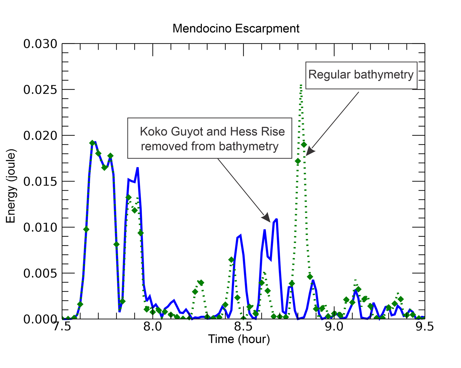
To partially address the role of KG and HR in organizing far-distance propagation, the bathymetry is modified by setting the depth to 4500 m to effectively remove their influence. The resulting plot (Figure 11) shows potential energy for the original bathymetry as a green dashed line with diamonds, while a blue line represents the potential energy for the modified bathymetry. The first group of waves arriving at the Mendocino Escarpment remains unchanged with the altered bathymetry, indicating that it travels along a route unaffected by either HR or KG. However, the last group of waves, which exhibits the strongest energy maximum, is entirely absent in the modified bathymetry. This result suggests that the late-arriving secondary tsunami signals are scattered from KG and guided by the elongated HR towards the Mendocino Escarpment. The approach of altering bathymetry, first introduced by Kowalik at al. (2008) to study energy fluxes near Crescent City, has proven helpful in this study for analyzing the influence of bathymetry on the generation of potential energy.

7. Koko Guyot interaction with Japan Tōhoku Tsunami

7.1. Energy evolution

To investigate the interaction of tsunamis with prominent bathymetric features and the development of the energy change generated by such interactions, the details of tsunami interactions with KG are analyzed.

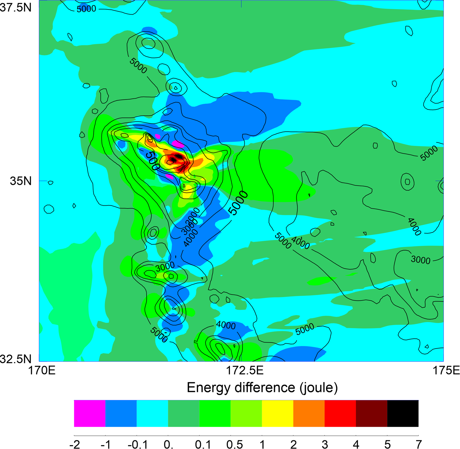
Analyzing the distribution of kinetic and potential energy provides further insight into the dynamics of tsunami interactions with KG. Two key parameters to consider are the dimensionless ratio $e_k/e_p$ and the dimensional difference $e_p-e_k$. Since these parameters fluctuate significantly at each time step, their maximum values over time are identified at each computational cell. Figure 12 illustrates the energy difference, showing that potential energy dominates over the seamount's summit, where strong sea level oscillations develop. In contrast, kinetic energy prevails along the seamount slope, where negative values are observed. The most significant differences occur at the central dome (6.5 joules), with smaller differences at the northwest (3.5 joules) and southeast (2.5 joules) domes. Both kinetic and potential energy follow the downstream wake pattern, directing energy toward HR.

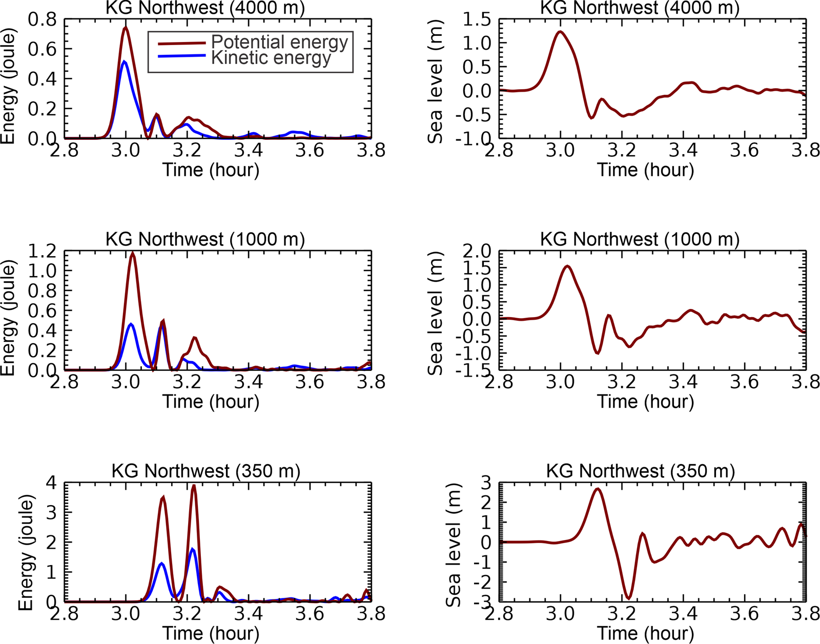
To capture the reflection dynamics during the initial interaction of the tsunami with the KG seamount; the processes that occur as the primary wave approaches from the northwest and propagates toward the northwest dome are analyzed. Figure 13 illustrates the time history of sea level and energy at three locations, starting from the shallowest point at the northwest dome of KG at a depth of 350 m, and two additional points located further northwest at depths of 1000 m and 4000 m. The energy differences in the positive wave increase from 0.24 joules at 4000 m, to 0.75 joules at 1000 m, and to 2.3 joules at 350 m (lefthand panels) while simultaneously, the sea level minimum drops from $-1$ m to $-3$ m. As the wave propagates into shallower waters, two distinct processes occur: the disparity between potential and kinetic energy grows in the positive wave, at the same time the negative portion is amplified and becomes dominant at the summit. This process notably influences wave reflection as the wave approaches the dome. The reflection coefficient $r_i$ begins at 0.19 at 4000 m, where the wave-seamount interaction initiates, and increases to 0.45 at both 1000 m and at 350 m. This final value closely matches the coefficient observed at the central dome of KG. A similar pattern is observed along the western and northern flanks, where the wave wraps around the central dome.

7.2. Wave evolution in time

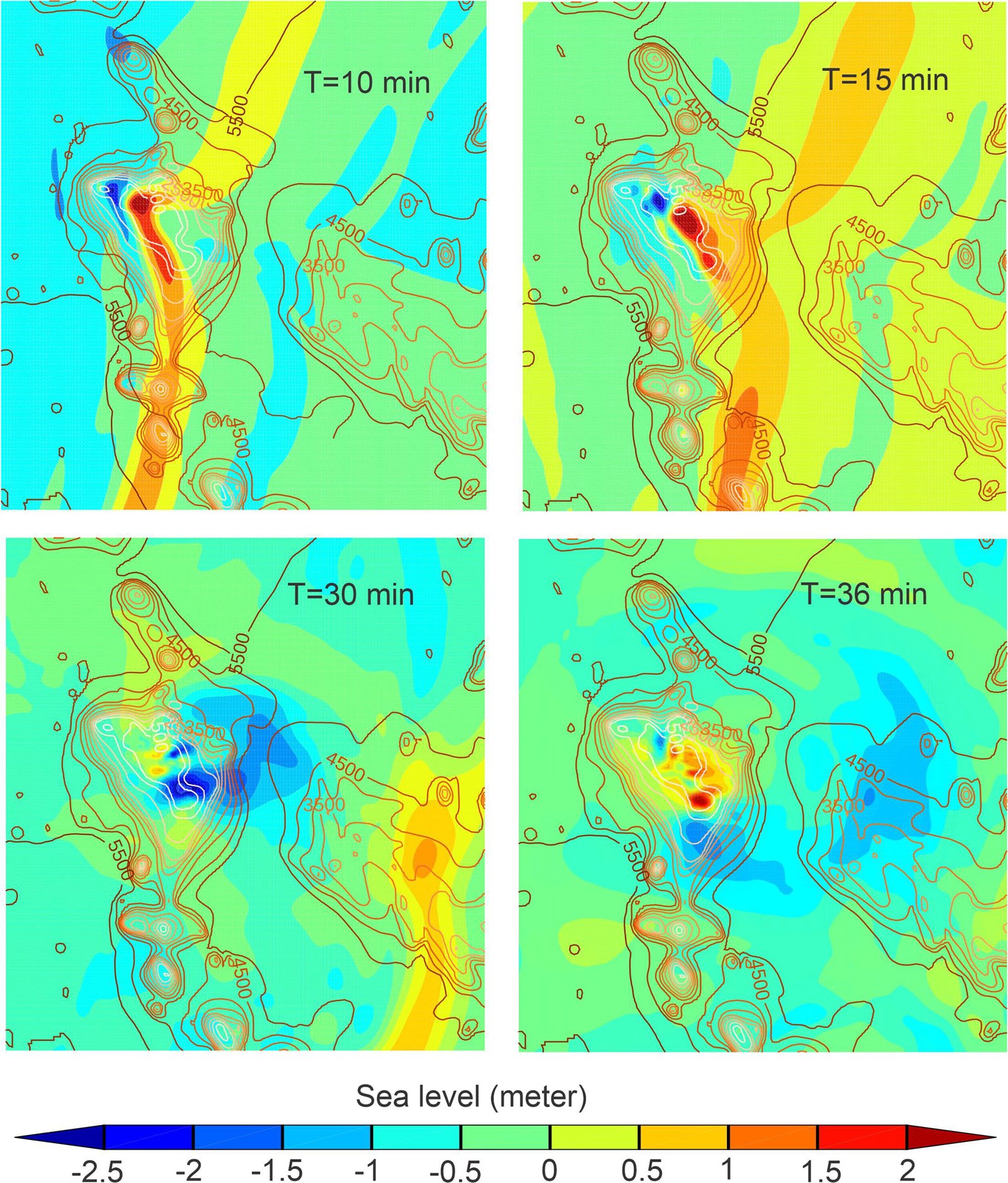
The short time history of sea level amplification caused by the Japan Tōhoku Tsunami is illustrated in the four panels of Figure 14. The first tsunami wave, arriving at the northwest flank of the seamount (upper left panel), slows down due to the shallow depth along the ridge. Following the positive wave (first wave), a blue domain representing the amplified negative signal appears and travels (as shown in the upper row of the panels) toward the center of KG. Primary tsunami amplification is driven by the interaction between the slowly moving wave along the ridge and the faster-moving waves in the deep ocean. This phenomenon is depicted in the upper row of Figure 14, where the steep slope of the seamount almost halts the tsunami wave. The wavefront bends and wraps around the seamount, resulting in a secondary interaction as the tsunami shoals along the less steep slopes. This interaction organizes a strong negative signal in the middle portion of the seamount (left panel in the lower row). Subsequently, a new wave is formed, shifting the source of the negative signal to the southern and eastern flanks of KG (lower right panel).

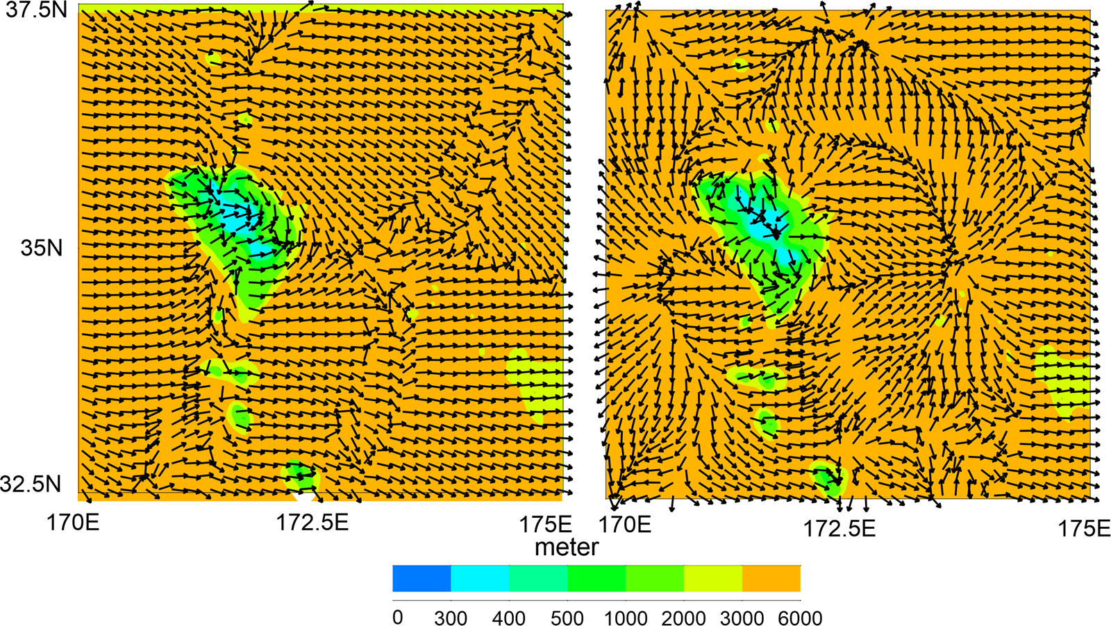
To support the conclusion that energy is concentrated at the seamount during the initial interaction stage and subsequently becomes the source of a new tsunami wave, two vector plots of energy flux are presented in Figure 15. These plots, taken at $t=10$ and 30 minutes after the wave's arrival at the northwest slope of the seamount, clearly demonstrate the initial concentration of energy and its later radiation. The transition from concentration to radiation occurs around 20 minutes, further emphasizing the role of the seamount as the source of the new tsunami wave.

7.3. Simplified case: Elliptical seamount

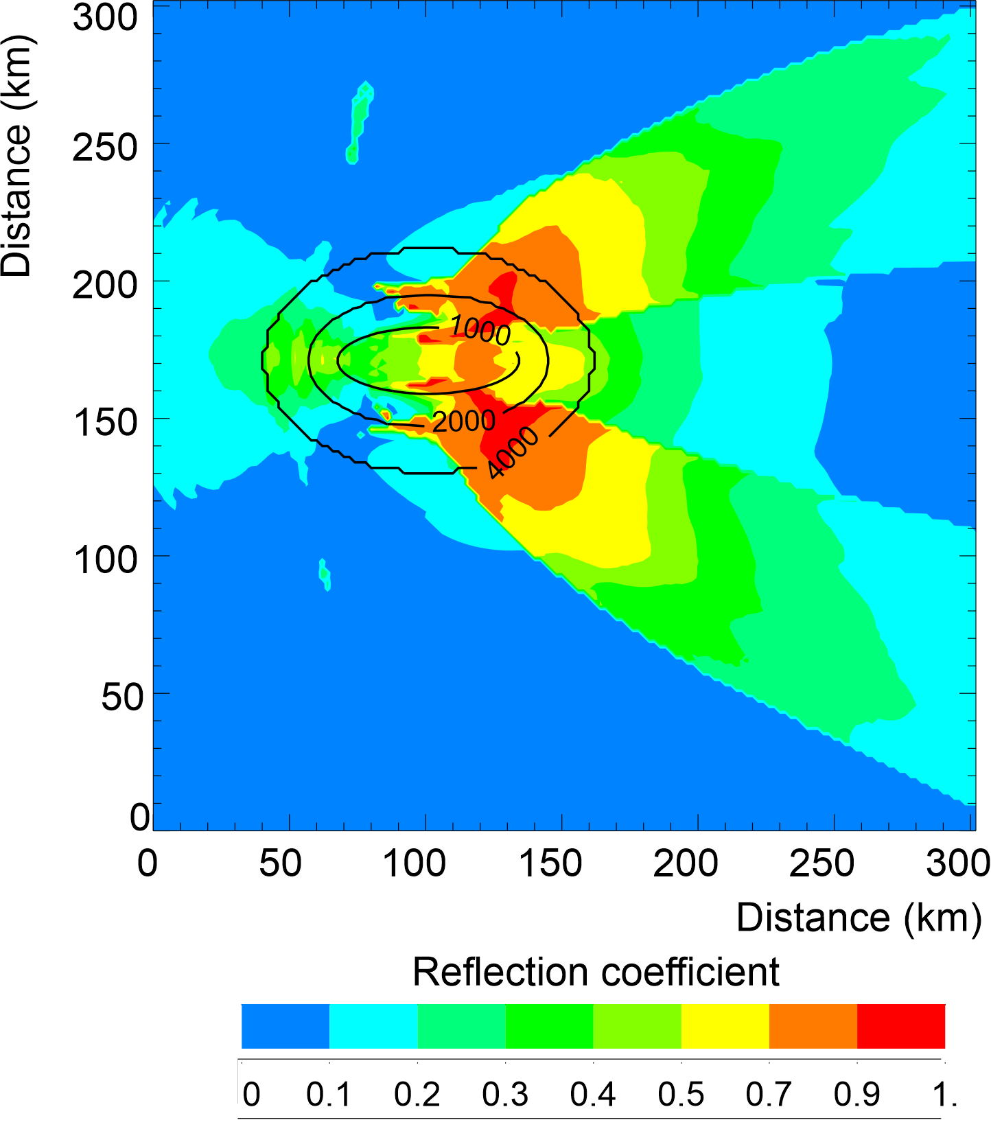
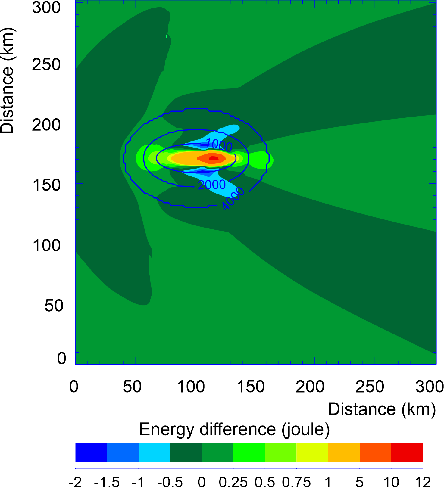
An elliptical seamount model is used to simplify the bathymetry of KG in order to reproduce and highlight key conclusions from the experiments described above. The base of the seamount lies at a depth of 4000 m and is represented by an ellipse with a semi-minor axis of 35 km and a semi-major axis of 55 km. Beyond the base, the depth remains constant at 4000 m. The summit, located at a depth of 400 m, is modeled by an ellipse with a semi-major axis of 27 km and a semi-minor axis of 10 km. In the computations, the distance between the grid points is 2 km.

As shown in Figure 14, the tsunami interacts with the KG seamount as it moves from the northwest flank to the southeast flank, following the seamount's elongated axis. In this simplified numerical experiment, a 20-minute sinusoidal wave with a 1 m amplitude propagates from the open boundary toward the ellipse's major axis to simulate this interaction. Figure 16 illustrates how energy and sea level respond in three different regions of the seamount, with notable amplification near the summit. The three test depths are located at grid points along the line falling on the semi-major axis. The broken green line represents the sinusoidal wave at the open boundary, showing a positive sea level at the wavefront. In the deep ocean domain, energy remains balanced between the positive and negative sea levels. On the upstream seamount slope (middle row), the wave interacts with the topography, amplifying both the crest and the trough, with the trough experiencing stronger amplification. This leads to the dominance of potential energy associated with the negative sea level, as shown in the left panel of the middle row. At the upstream summit of the seamount (lower row, left panel), the highest peaks in both potential and kinetic energy occur, accompanied by a significant difference in sea level between the wave crest and trough (lower row, right panel). The trough causes a sharp drop in water column height, increasing potential energy. After the sinusoidal wave passes, the summit exhibits partially trapped and radiated oscillations that gradually dissipate over time. These processes, depicted in Figure 16, closely resemble those observed at the northwest dome of KG Figure 13, lower panel), showing similar patterns of sea level amplification and energy behavior.

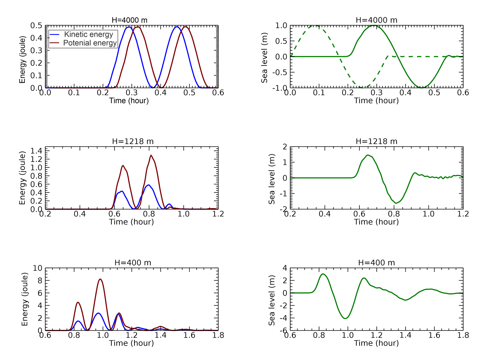
Experiments with the simplified elliptical seamount reveal its reflective properties using Eq. (14). In the deep domain, $r_i$=0, on the slope ($H=1218$ m) $r_i$=0.4 for the crest and 0.37 for the trough; and at the top ($H=400$ m), $r_i$=0.5 for the crest and 0.45 for the trough. These values align closely with the coefficients calculated for the KG seamount. This approach appears to effectively capture the initial interactions of a wave with the upstream summit of the elliptical seamount.

Figure 17 shows the reflection coefficient pattern across the entire seamount. These are the maximum values attained over time at each computational cell. The initial interaction between the wave and the seamount produces reasonable values of the reflection coefficient, particularly on the upstream slope of the seamount. However, as the wave, with its established energy differences, continues to interact with the seamount, these differences are amplified by dynamic processes occurring at and around the seamount. Consequently, neither the downstream pattern nor the high reflection coefficient values in this region can be attributed solely to reflection processes. Further insight into tsunami-seamount interactions can be obtained by analyzing the differences between potential and kinetic energy. Unlike the reflection coefficient, which uses the absolute value of the energy difference (see Eq. (16)), it is also possible to examine both the positive and negative maximum values over time at each computational cell. Figure 18 illustrates the maximum energy difference, revealing that potential energy dominates over the seamount's summit, where strong sea level oscillations develop, particularly near the right focal point of the elliptical pattern. In contrast, kinetic energy prevails along the seamount slope, aligning with the downstream wake patterns. Therefore, the distribution of large reflection coefficient values in the downstream field is closely linked to the amplification of potential and kinetic energies in this region.

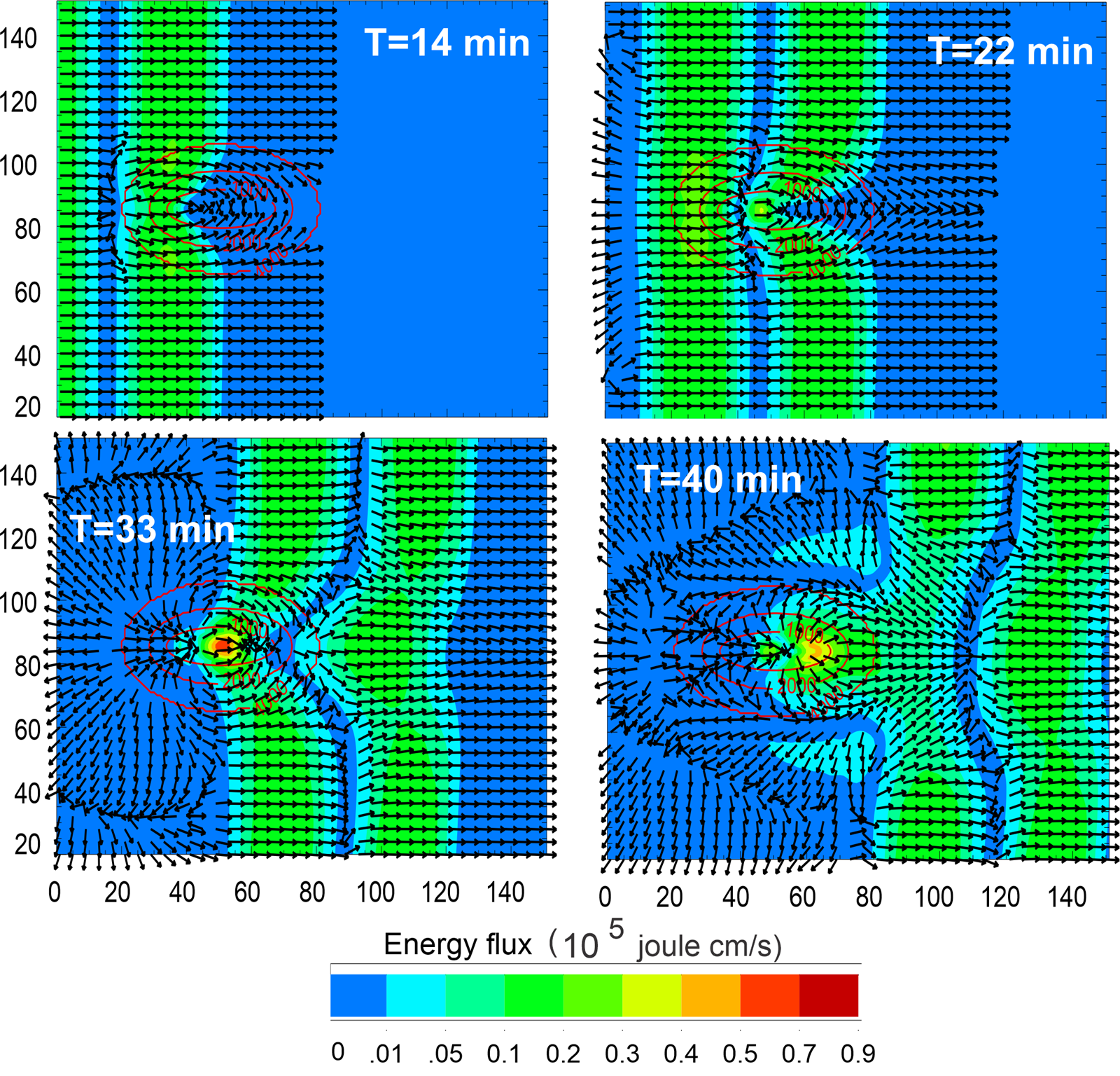
To better understand the changes in the upstream reflection coefficients, the energy fluxes associated with the wave as it propagates over the seamount are analyzed. Figure 19 illustrates the temporal evolution of energy flux over the seamount in four panels. At 14 minutes, the wavefront approaches the seamount. While the energy flux magnitude remains relatively low, the seamount causes energy reflection by the upstream slope and energy concentration towards the downstream slope. By 22 minutes, as the wave reaches the vicinity of the seamount, the energy flux vectors begin to deflect and curve around the elliptical mountain, indicating a tendency for energy to concentrate over the seamount. At 33 minutes, during the passage of the second half-wave (negative sea level), the interaction intensifies. The highest energy flux values (depicted in yellow to red colors) occur near the seamount's summit, signaling energy convergence. At the same time, the energy flux vectors show significant deflection and divergence away from the summit, with minimal energy directed upstream and a larger flux directed downstream. At 40 minutes, after the wave has passed over the seamount, the energy flux vectors form a complex pattern downstream. High energy flux regions are concentrated near the lee side of the seamount, while weaker fluxes persist farther away. The interaction between the wave and the seamount significantly alters the wave's energy distribution, creating regions of focused energy and distinctive downstream wake patterns. These energy-driven dynamics are also reflected in the downstream distribution of the reflection coefficient, as shown in Figure 17.

8. Conclusions and discussion

This study demonstrates a new approach to investigate the interaction of tsunamis with bathymetry that focuses on local energy equilibrium. By decomposing the tsunami energy into kinetic and potential components, a new reflection coefficient based on the local energy imbalance is introduced. The energy equilibrium at specific points and times is analyzed, starting with a simplified channel model that features a depth discontinuity. Extending this analysis to the 2011 Japan Tōhoku Tsunami, we find that while energy equilibrium is maintained across vast ocean distances, it is disrupted at KG. Prior investigations (e.g., Yoon et al., 2014; Tang et al., 2012; Kowalik et al., 2008) primarily employ energy flux or amplitude-based amplification factors to study similar phenomena. In contrast, we introduce energy imbalance as a distinct metric, thereby yielding a refined understanding of the spatial and temporal dynamics of tsunami energy in the vicinity of complex bathymetry. Using a simplified elliptical seamount model resembling KG, key patterns of wave amplification observed in the Tōhoku Tsunami 2011 are confirmed. These experiments also show that proper application of the reflection coefficient is most relevant during the initial interaction between the incoming wave and the seamount. As the wave, with its initial energy difference, continues to interact with the seamount, this difference becomes amplified by dynamic processes occurring at and around the feature. The amplified difference then propagates downstream, forming a wake pattern. The role of topography in tsunami energy transformation is well studied, particularly by Kim and Son (2018), who analyze how tsunami waves evolve over the continental slope and shelf. To this end, energy, mass, and momentum are integrated at each time step along the wave's propagation path. Their results are consistent with this work, indicating that energy transformation is particularly significant on steep continental slopes, while potential and kinetic energies remain balanced on the shelf until wave breaking occurs. The reflective properties of bathymetric features are studied analytically by Mofjeld et al. (2000). They introduce a scattering index based on the depths at the top and base of bathymetric features. For KG, the scattering index is consistent with the reflection coefficient calculated in this study. While Mofjeld et al. (2000) examined the amplitudes of incident, reflected, and transmitted waves, we introduce energy interference patterns between the incident and reflected waves. A key parameter in both the scattering index and the reflection coefficient is the horizontal dimension of the bathymetric feature relative to the wavelength (L) of the incoming wave. With a horizontal dimension of roughly 100 km, KG falls within the wavelength range typical of tsunami periods. To examine KG's interaction with waves of varying periods, a sinusoidal wave with a 1 m amplitude and periods ranging from 5 to 60 minutes is sent toward the seamount. The results indicate that the wave amplitude at the summit significantly increases—by up to four times—around a 20-minute period. Shorter waves (L $\simeq$ 60 km, period 5 min) are strongly reflected, while longer waves (L $>$ 600 km, period 50 min) exhibit high transmissivity, suggesting minimal interaction with KG. The concepts of potential and kinetic energy, though applied here to wave reflection, have broader significance. Tracking energy imbalances clarifies tsunami dynamics by distinguishing regions of kinetic (high velocities) and potential (large sea levels) energy dominance. This approach links tsunami observations and models to the fundamental concept of energy, with the ratio $e_k/e_p$ and the difference $e_p-e_k$ serving as useful diagnostic tools.

Acknowledgements

I am indebted to Dr. Dmitry Brazhnikov (University of Alaska), Dr. Juan Horrillo (Texas A&M University), and William Knight (Alaska Tsunami Warning Center) for their thorough comments and many valuable suggestions that strengthened this paper. I also extend my gratitude to the reviewers for their insightful comments and recommendations, which further improved the manuscript.

Conflict of interest

The author declares that he has no known competing financial interests or personal relationships that could have appeared to influence the work reported in this paper.

References

• Abadie, S. M., Harris, J. C., Grilli, S. T., Fabre, R., 2012. Numerical modeling of tsunami waves generated by the flank collapse of the Cumbre Vieja Volcano (La Palma, Canary Islands): Tsunami source and near field effects. J. Geoph. Res. 117, C05030. https://doi.org/10.1029/2011JC007646
• Dutykh, D., Dias, F., 2009. Energy of tsunami waves generated by bottom motion. Proc. R. Soc. A. 465, 725–744. https://doi.org/10.1098/rspa.2008.0182
• Fine, I. V., Kulikov, E. A., Cherniawsky, J. Y., 2013. Japan's 2011 Tsunami: Characteristics of wave propagation from observations and numerical modelling. Pure Appl. Geophys. 170, 1295–1307. https://doi.org/10.1007/s00024-012-0555-8
• Horrillo, J., Knight, W., Kowalik, Z., 2012. Tsunami propagation over the North Pacific: Dispersive and nondispersive models. Sci. Tsunami Hazards. 31 (3), 154–177.
• Horrillo, J., Knight, W., Kowalik, Z., 2021. Numerical Modeling of Tsunami Waves. Advanced Series on Ocean Engineering, World Sci. Publ., Singapore, 412 pp. https://doi.org/10.1142/12421
• Kim, D-H., Son, S., 2018. Lagrangian-like volume tracking paradigm for mass, momentum and energy of nearshore tsunamis and damping mechanism. Sci. Rep. 8 (1), 14183–14194. https://doi.org/10.1038/s41598-018-32439-6
• Koshimura, S., Hayashi, Y., Munemoto, K., Imamura, F., 2008. Effect of the Emperor seamounts on trans-oceanic propagation of the 2006 Kuril Island earthquake tsunami. Geophys. Res. Lett. 35, L02611. https://doi.org/10.1029/2007GL032129
• Kowalik, Z., Knight, W., Logan, T., Whitmore, P., 2005. Numerical modeling of the global tsunami: Indonesian tsunami of 26 December 2004. Sci. Tsunami Haz. 23 (1), 40–56.
• Kowalik, Z., 2008. Energy flux as a tool in locating tsunami secondary sources. Sci. Tsunami Haz. 27 (3), 1–29.
• Kowalik, Z., Horrillo, J., Knight, W., Logan, T., 2008. Kuril Islands tsunami of November 2006: 1. Impact at Crescent City by distant scattering. J. Geophys. Res. 113, C01020. https://doi.org/10.1029/2007JC004402
• Kowalik, Z., Murty, T.S., 1993. Numerical Modeling of Ocean Dynamics, World Sci. Publ., Singapore, 481 pp. https://doi.org/10.1142/1970
• Lamb, H., 1945. Hydrodynamic, 6th edn., Dover Publ., New York, 738 pp.
• Levin, B.W., Nosov, M., 2015. Physics of Tsunamis, Springer Internat. Publ., 388 pp. https://books.google.com/books?id=CADOCgAAQBAJ
• Li, Y., 2000. Tsunamis: Non-Breaking and Breaking Solitary Wave Run-Up. Caltech, Pasadena, 219 pp. https://doi.org/10.7907/Z9G44N7F
• Lopez-Venegas, A.M., Horrillo, J., Pampell-Manis, A., Huerfano, V., Mercado, A., 2014. Advanced tsunami numerical simulations and energy considerations by use of 3D–2D coupled models: The October 11, 1918, Mona Passage Tsunami. Pure Appl. Geophys. 172, 1679–1698. https://doi.org/10.1007/s00024-014-0988-3
• Marchuk., An. G., 2022. Capturing of the tsunami wave energy by islands. Bull. Nov. Comp. Center, Math. Model. in Geoph., 24, 15–25.
• Mei, C.C., Stiassnie, M., Yue, D.K.-P., 2005. Theory and Applications of Ocean Surface Waves, Part 1: Linear Aspects, World Scientific, Advanced Series on Ocean Engineering, Singapore, 506 pp. https://doi.org/10.1142/5566
• Mofjeld, H.O., Titov, V.V., Gonzalez, F.I., Newman, J.C., 2000. Analytic Theory of Tsunami Wave Scattering in the Open Ocean with Application to the North Pacific. NOAA Technical Memorandum OAR PMEL-116, Seattle, 38 pp.
• Mofjeld, H.O., Titov, V.V., Gonzalez, F.I., Newman, J.C., 2001. Tsunami scattering provinces in the Pacific Ocean. Geoph. Res. Letters. 28, 335–338. https://doi.org/10.1029/2000GL011710
• Munk, W.H., 1963. Some comments regarding diffusion and absorption of tsunamis. [In:] Cox, D.C., (Ed.), Proc. Tsunami Meetings Associated with the Tenth Pacific Science Congress, Honolulu, Hawaii, Aug.-Sept. 1961. IUGG Monograph, Paris, 53–72.
• Nekrasov, A.V., 1992. On tidal energy horizontal circulation. J. Korean Soc. Coast. Ocean Eng. 4 (3), 168–177.
• Okada, Y., 1985. Surface deformation due to shear and tensile faults in a half-space. Bull. Seismol. Soc. Am. 75, 1135–1154.
• Okal, E. A., 2021. The energy of a tsunami generated by dynamic uplift of the ocean bottom. I. Analytical solutions. Pure Appl. Geophys. 178, 4985–4999. https://doi.org/10.1007/s00024-021-02804-0
• Rabinovich, A.B., Candella, R.N., Thomson, R.E., 2013. The open ocean energy decay of three recent trans-Pacific tsunamis. Geoph. Res. Letters. 40 (12), 3157–3162. https://doi.org/10.1002/grl.50625
• Tang, L., Titov, V. V., Bernard, E.N., Wei, Y., Chamberlin, C.D., Newman, J.C., Mofjeld, H.O., Arcas, D., Eble, M.C., Moore, C., Uslu, B., Pells, C., Spillane, M., Wright, L., Gica, E., 2012. Direct energy estimation of the 2011 Japan Tsunami using deep-ocean pressure measurements. J. Geoph. Res. 117, C08008. https://doi.org/10.1029/2011JC007635
• Yoon, S.B., Kim, S.C., Baek, U., Bae, J.S., 2014. Effect of bathymetry on propagation of tsunamis towards the East Coast of Korea. [In:] Green, A.N., Cooper, J.A.G. (Eds.), Proceedings 13th International Coastal Symposium (Durban, South Africa), J. Coast. Res., Sp. Iss. 70, 332–337.
• Zhao, X., Wang, B., Liu, H., 2012. Characteristics of tsunami motion and energy budget during runup and rundown processes over a plane beach. Physics of Fluids. 24 (6), 062107. https://doi.org/10.1063/1.4729597